An R function: OLS/Robust scaled mass index

R code

	# Inspired by Peig & Green
	# "New perspectives for estimating body condition from mass/length data:
	# the scaled mass index as an alternative method"
	# Oikos 118: 1883-1891, 2009
	# Author: Chen-Pan Liao
	scaledMassIndex <-
	function(x, y, x.0 = mean(x)) {
	require(smatr)
	require(magrittr)
	require(MASS)
	require(data.table)
	logM.ols <- lm(log(y) ~ log(x))
	logM.rob <- rlm(log(y) ~ log(x), method = "M")
	b.msa.ols <- coef(sma(log(y) ~ log(x)))[2]
	b.msa.rob <- coef(sma(log(y) ~ log(x), robust = T))[2]
	SMI.ols <- y * (x.0 / x) ^ b.msa.ols
	SMI.rob <- y * (x.0 / x) ^ b.msa.rob
	res <- data.frame(SMI.ols, SMI.rob, x, y)
	pred.DT <-
	data.table(x = seq(min(x), max(x), length = 100)) %>%
	.[, y.ols := predict(logM.ols, newdata = .) %>% exp] %>%
	.[, y.rob := predict(logM.rob, newdata = .) %>% exp]
	attr(res, "b.msa") <- c(ols = b.msa.ols, rob = b.msa.rob)
	return(res)
	}

view raw robust-scaledMassIndex.R hosted with ❤ by GitHub

Example

library(magrittr)
library(data.table)
library(ggplot2)
library(ggpubr)
set.seed(123)
dt <-
  data.table(`Body length` = seq(1, 5, 0.5)) %>%
  .[, `Body weight` := 2 * `Body length` ^ (3 + rnorm(length(`Body length`), sd = 0.001))] %>%
  rbind(., data.table(`Body length` = 6, `Body weight` = 200)) %>%
  .[order(`Body length`), ]

dt.SMI <-
  scaledMassIndex(dt$`Body length`, dt$`Body weight`, x.0 = 2)
summary(dt.SMI)

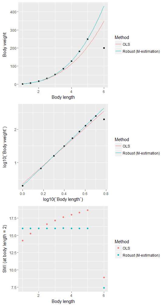
g1 <-
  ggplot(dt, aes(`Body length`, `Body weight`)) +
  geom_point() +
  geom_line(aes(x, y, color = Method),
            data = attr(dt.SMI, "pred") %>% melt(., "x", c("y.ols", "y.rob"), "Method", "y")) +
  scale_colour_discrete(labels = c("OLS", "Robust (M-estimation)"))
g2 <-
  ggplot(dt, aes(log10(`Body length`), log10(`Body weight`))) +
  geom_point() +
  geom_line(
    aes(log10(x), log10(y), color = Method),
    data = attr(dt.SMI, "pred") %>% melt(., "x", c("y.ols", "y.rob"), "Method", "y")
  ) +
  scale_colour_discrete(labels = c("OLS", "Robust (M-estimation)"))
g3 <-
  ggplot(melt(dt.SMI, "x", c("SMI.ols", "SMI.rob"), "Method"),
         aes(x, value)) +
  geom_point(aes(color = Method)) +
  xlab("Body length") +
  ylab("SMI (at body length = 2)") +
  scale_colour_discrete(labels = c("OLS", "Robust (M-estimation)"))
ggarrange(g1,
          g2,
          g3,
          ncol = 1,
          nrow = 3,
          align = "hv")