One-dimensional interpolation with R

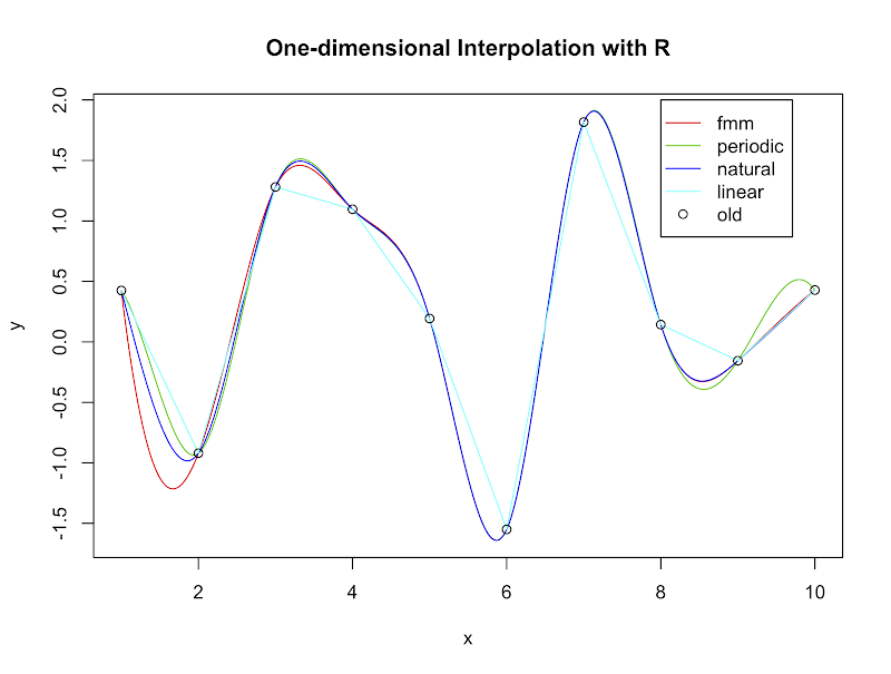
The function approx() and spline() provide one-dimensional linear and non-linear interpolation with R, respectively. Syntax of them are similar, for example,

x.old <- 1:10
y.old <- rnorm(10)
x.new <- seq(1, 10, 0.001)

# Linear interpolation
y.new.linear <- approx(x.old, y.old, xout = x.new)$y

# Forsythe, Malcolm and Moler's spline (default of spline)
y.new.fmm <- spline(x.old, y.old, xout = x.new, method = "fmm")$y

# Natural splines
y.new.natural <- 
  spline(x.old, y.old, xout = x.new, method = "natural")$y

# Periodic splines 
y.new.periodic <-
  spline(x.old, y.old, xout = x.new, method = "periodic")$y

# Plot
plot(
  y.new.fmm ~ x.new,
  type="l", col=2, xlab="x", ylab="y",
  main="One-dimensional Interpolation with R"
)
lines(y.new.periodic ~ x.new, col=3)
lines(y.new.natural ~ x.new, col=4)
lines(y.new.linear ~ x.new, col=5)
points(y.old ~ x.old)
legend(8, 2, c("fmm", "periodic", "natural", "linear", "old"),
  col = c(2:5,1), lty = c(1,1,1,1,0), pch = c(NA,NA,NA,NA,1), merge = T
)

One-dimensional Interpolation with R

Nested ANOVA permutation test in R

A R function for the permutation test for onw-way nested design ANOVA.

This work is inspired by Dr. David C. Howell, University of Vermont. In Dr. Howell’s webpage “Permutation Tests for Factorial ANOVA Designs” (http://www.uvm.edu/~dhowell/StatPages/More_Stuff/Permutation%20Anova/PermTestsAnova.html [access on May 28, 2012]), he described the algorithm of permutation test for a one-way nested design ANOVA by using R language. I followed this algorithm and made a R function to do this test.

Example

dat <- read.csv(textConnection("
 trt , unit , obs
 1 , 1 , 11
 1 , 1 ,  9
 1 , 1 ,  9
 1 , 2 ,  8
 1 , 2 ,  7
 1 , 2 ,  6
 1 , 3 ,  8
 1 , 3 , 10
 1 , 3 , 11
 2 , 4 , 11
 2 , 4 ,  8
 2 , 4 ,  7
 2 , 5 , 10
 2 , 5 , 14
 2 , 5 , 12
 2 , 6 ,  9
 2 , 6 , 10
 2 , 6 ,  8
"))

## traditional nested ANOVA
mod.2 <- aov(
 obs ~ factor(trt) + Error(factor(unit)),
 data = dat
)
summary(mod.2) # alternative

## permutation nested ANOVA
nestedPermutationAnova(dat$obs, dat$trt, dat$unit, 499)

Logistic regression with package rms in R

The rms package by Frank E Harrell Jr provides a useful function lrm to apply logistic regression. Moreover, this function also provides many useful statistics, and a gooeness-of-fit test (le Cessie and Houwelingen test) could be applied by using the function residuals(a lrm model, "gof"). Read the official document of package rms for more details.

淺談貝氏定理

本文將介紹貝氏定理 (Bayes’ theorem) 的推導與實例。

推導

條件機率的定義是, \[ \Pr(A|B)= \frac{\Pr(A \cap B)}{\Pr(B)}, \] 其中 $\Pr(A|B)$ 是指在事件 $B$ 發生的前題下, 事件 $A$ 發生的機率; $\Pr(A \cap B)$ 是指事件 $A$ 發生且事件 $B$ 發生的機率. 當然, $A \cap B$ 與 $B \cap A$ 是完全同義的, 因此, 我們也可以得到 \[ \Pr(B|A)=\frac{\Pr(B \cap A)}{\Pr(A)}=\frac{\Pr(A \cap B)}{\Pr(A)}. \]

有趣的事發生了. 若將上述二式中的 $\Pr(A \cap B)$ 單離出來, 可以發現 \[ \Pr(A \cap B) = \Pr(A|B) \times \Pr(B) = \Pr(B|A) \times \Pr(A), \] 可得 \[ \Pr(A|B) = \frac{\Pr(B|A) \times \Pr(A)}{\Pr(B)}, \] 被稱為貝氏定理. 不過在實用上來說, 常利用全機率定理改寫分母, 成為定理的另一個形式 \[ \Pr(A|B) = \frac{\Pr(B|A) \times \Pr(A)}{\Pr(B|A)\times \Pr(A) + \Pr(B|\lnot A)\times \Pr(\lnot A) }, \] 其中 $\lnot A$ 表示 “非 $A$”.

例題

Wikipedia 中描述了一個貝氏定理中著名的 “吸毒測試” 例題, 簡單翻譯與修改後如下. 某種檢測吸毒的方法具有 99% 的敏感度和 97% 的可靠度, 也就是有吸毒者受測呈陽性的機率為 99% 而非吸毒者受測呈陰性的機率是 97%. 調查人員已經知道某群體的總體吸毒率為 0.1%. 已知, 在該群體中某一位人員受檢後呈陽性, 則該人員吸毒的機率是多少?

令吸毒事件為 $D$, 測試結果呈陽性為 $P$. 由命題可知, $\Pr(P|D)=0.99$, $\Pr(\lnot P|\lnot D)=0.97$, $\Pr(D)=0.001$. 由貝氏定義可知, \[ \begin{aligned} \Pr(D|P) =& \frac{\Pr(P|D) \times \Pr(D)}{\Pr(P)} \\ =& \frac{\Pr(P|D) \times \Pr(D)}{\Pr(P|D) \times \Pr(D) + \Pr(P|\lnot D) \times \Pr(\lnot D)} \\ =& \frac{\Pr(P|D) \times \Pr(D)}{\Pr(P|D) \times \Pr(D) + [1-\Pr(\lnot P|\lnot D)] \times [1-\Pr(\lnot D)]} \\ =& \frac{0.99 \times 0.001}{0.99 \times 0.001 + (1-0.97) \times (1-0.001)} \\ \simeq& 0.032 \end{aligned} \] 為所求, 也就是該人員受測呈陽性但有吸毒的機率只有 3.2%, 即使該檢測有 99% 的敏感度. 這種結果是不是與你預期的差距很大?

利用貝氏定理, 統計學家已經將之推廣出一派新的統計學門, 稱為貝氏推論. 貝氏推論的核心概念是, 在已知的資料中, 如何從過去的知識推論母體. 在例題中, 過去的知識 $\Pr(D)$ 被稱為事前機率 (prior), $\Pr(D|P)$ 被稱為事後機率 (posterior), 而 $\Pr(P|D) / \Pr(P)$ 被稱為標準概似度 (standardised likelihood). 因此, 貝氏定理亦常被表示成 \[ \text{posterior} = \text{standardised likelihood} \times \text{prior}. \] 假如 posterior 不易取得, 可藉由對 prior 更多的了解, 使我們可以更有信心地推論 posterior, 是貝氏推論的重要武器.